Natural and climatic anomalies in the Northern hemisphere and their impact on the economy

Dmitry SOLOVYEV
JIHT RAS, IO RAS, Moscow, Russia,
Candidate of Physical and Mathematical Sciences
e-mail: solovev@guies.ru

Introduction

The beginning of the 21st century was marked by a number of major natural, climatic, man-made, social, financial, economic and virological disasters. Suffice it to recall the accelerated increase in global temperature in the Northern Hemisphere with the onset of the millennium, the explosion of a volcano in Iceland, Hurricane Katrina, the accident at the Fukushima nuclear power plant, floods and forest fires in southern Europe and Siberia, color revolutions in the Arab world, economic crises in 1998-1999 and 2009 [1]. And finally, the global world crisis in 2020, triggered by the coronavirus pandemic [2], [3]. The coincidences are too numerous to be explained by chance – including the fact of their concentration in time. The frequency of these events coincides with the beginning of the 2000s, at the turn of the first and second decades, and at the beginning of the present time [4].

Analyzing the statistical data of anomalous natural, political and economic phenomena, it can be noted that all crisis events have in their temporal dynamics the manifestation of a certain cyclicality, largely due to periodic natural processes [5].

Analysis and forecast of the cyclical nature of climatic phenomena and indicators of economic development

For a detailed analysis of the spectral characteristics of various curves of natural and economic dynamics, the methods of spectral analysis were applied, which make it possible to identify the main statistical regularities of these phenomena and their comparison with the corresponding parameters of the economy (GDP). In particular, a study was conducted of the temporal relationship between the main dominant global natural factors – the temperature anomalies of the Northern Hemisphere (Tnh), the Arctic zone (Tarct), the global number of natural anomalies (NA), and financial and economic processes (using the example of the GDP of the world’s largest economy – the United States). The curves are plotted for the interval of 1900-2020 with further expansion until 2030-2050, due to the inclusion in the actual data series of the forecast obtained using the neural model of the Institute of Energy Strategy [4], [6], [7]. It’s important to note that due to the high number of interrelated factors on the market, the neural model used allows for “mixing” other parallel inputs, thereby taking into account the influence of correlated processes.

As the input for the year-to-year variation of the air temperature anomalies in the Arctic region (for the latitudinal zone of 60-90° N) and the Northern Hemisphere of the Earth (for the latitudinal zone of 0-90° N), we used the mean monthly air temperatures near the Earth’s surface averaged over the corresponding latitudinal zone (Tnh and Tarct curves) obtained from the Climate Research Department “Berkeley Earth” (BE) of the University of East Anglia (these data are freely available at http://berkeleyearth.org/data/). The period of 1951-1980 was taken as the base averaging period for assessing air temperature anomalies; the methodology and algorithms for data processing and quality control at all stages are described in [8]. The input data for the US GDP and the global number of natural anomalies (NA) were obtained from the open archive of the laboratory of global changes in the data of the University of Oxford “Our World in Data” (OWID), available at: https://ourworldindata.org [9].
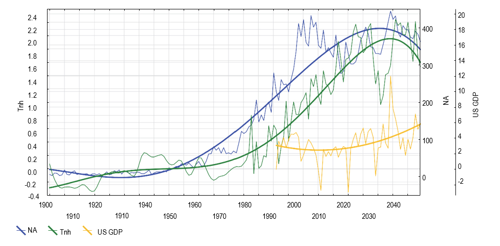
Fig. 1 shows the curves of Tnh, NA and US GDP as a function of time for 1900-2030 against the backdrop of the corresponding trend lines. From this graph, we can draw the preliminary conclusion that natural factors (Tnh and NA) have similar characteristics of trend lines, which indicates the presence of a possible more pronounced correlation between the time series values of Tnh and NA than Tnh and US GDP.
To confirm this assumption, an in-depth correlation analysis of these curves was carried out using three-dimensional (3M) and two-dimensional scatter diagrams.
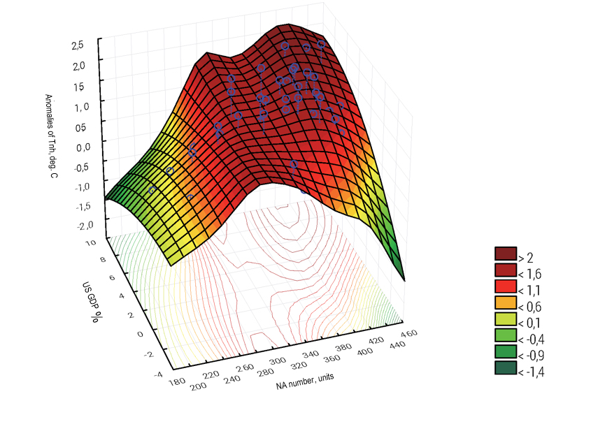
On the 3M-surface plot of average annual values of Tnh, NA and US GDP for 1900-2030 (Fig. 2.), it can be seen that the 3M-surface for anomalous temperatures of the Northern Hemisphere, plotted relative to the Z-axis (Tnh), has a more pronounced irregularity along the X-axis (NA) and is less pronouncedly curved along the Y-axis (US GDP) in the range of average values of the variables in question. At the same time, the growth of temperature anomalies – the “red area” of the surface – is typical for areas with a high number of natural anomalies and high GDP growth rates. This visual assessment confirms our preliminary conclusion about a more pronounced dependence of the temperature anomalies in the Northern Hemisphere on the increase in the number of natural anomalies. It is important to note, however, that there is also a visually-observed, statistically-significant relationship between “global warming” and US GDP growth.
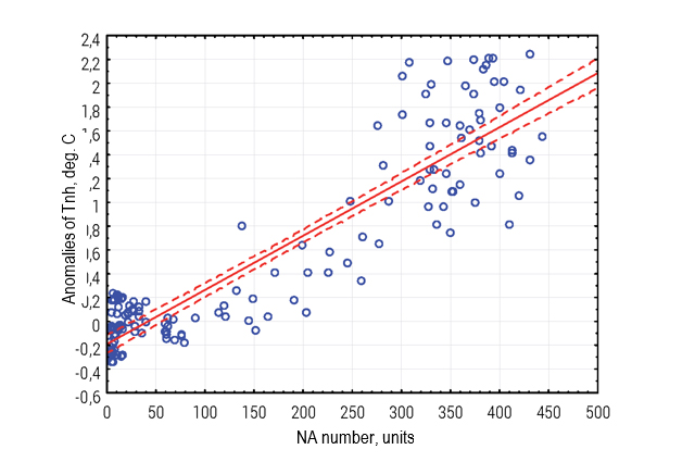
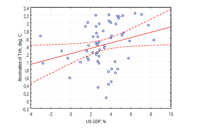
To identify quantitative correlations, the corresponding scatter diagrams were built (Fig. 3 and Fig. 4). The obtained diagrams confirm our assumption about the existence of a significant direct correlation between Tnh and NA (with a correlation coefficient of R = 0.54) and a less pronounced dependence of Tnh anomalies on US GDP (R = 0.27); see scatter diagrams in Fig. 3-5.

Comparative forecast dynamics of temperature anomalies in the Northern Hemisphere and the Arctic

One of the most important natural factors of dynamic development is the global climatic regime, determined by the curves of temperature fluctuations. To assess long-term temperature fluctuations on a global scale, temperature anomalies are calculated, which represent the deviation from the average or baseline temperature. Temperature anomaly is the deviation of the temperature of a given location (latitude and longitude), average daily, monthly, etc., from the corresponding long-term value (average or baseline temperature). Positive anomalies indicate that the observed temperature was above the baseline, while a negative anomaly indicates that the observed temperature was below the baseline. Since the 1980s, the deviation of the annual temperature from the mean values for the 20th century has been consistently positive. Temperature anomalies are usually more important in the study of climate change than absolute temperature. This is due to the fact that when calculating average absolute temperatures, factors such as station location and altitude can have a decisive influence on absolute temperatures, but are less significant in calculating anomalies.

As part of the preparation of historical data with parameter calibration to build up a multi-axis image and its subsequent use in a package neural model, a calibration forecast of Tnh and Tarct anomalies was carried out until 2050, including a forecast mixing a combination of various factors responsible for natural, social and economic processes.
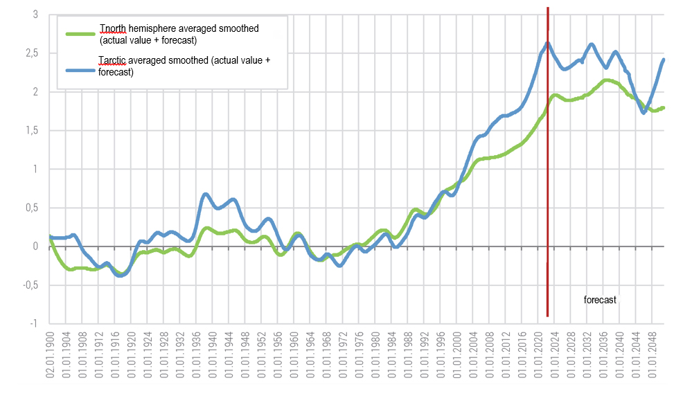
Fig. 5 shows the comparative temporal dynamics of the two curves of Tnh and Tarct anomalies for the period from 1901 to 2050.
The graphs show that global warming is occurring unevenly, with pauses. In addition, temperature changes in the Arctic itself are more volatile than in the entire Northern Hemisphere, apparently due to the scale of the territories. Global climate change can be viewed as a synthesis of natural and man-made factors. Natural year-to-year fluctuations occur chaotically, but a rhythm with a period of about 60 years is observed. Man-made factors determine the secular trend. During this time, the average temperature on the Earth has increased by 0.8 °C. These changes seem insignificant, but the environment is already reacting – for example, the level of the World Ocean has risen by 20 cm.
The Arctic temperature anomaly curve is one of the strongest indicators of climate change in this region over the past 50 years [10]. Over the past five decades (2015-2020), there has been a strong positive trend towards the warming of the Arctic climate (Fig. 5). This warming has considerably affected the Arctic cryosphere, primarily through a decrease in sea ice extent during the annual cycle, a decrease in the mass balance of ice sheets and glaciers, and an increase in permafrost temperatures. Ecosystems in the region are also very sensitive to temperature trends and extreme natural events. Changes in the Arctic environment caused by warming have been particularly pronounced over the past 15 years.
At the same time, the results of neural prediction of the long-term dynamics of the Tnh and Tarct anomaly curves show that by 2050, the growth of temperature anomalies will stabilize at an average level, which is characteristic for today, and may slow down, demonstrating a downward trend. This result was obtained on the basis of the use of algorithms of the “mixing” and inclusion in the calibration forecast of astronomical factors (the level of solar activity), economic dynamics (GDP), and the dynamics of the consumption of primary energy resources.
Climate change affects the entire world, including society. Global warming is associated with problems of providing the population with water, energy, food and healthcare, as well as with geopolitical problems.
At the same time, it should be borne in mind that the above curves of Tnh and Tarct temperature anomalies do not coincide with the targets of the Paris Climate Agreement – to keep the global average temperature rise well below 2°C and make efforts to limit the temperature rise to 1.5°C. This is due to different methods for assessing the degree of global warming. In the Paris Agreement, the global average temperature of the Earth’s surface refers to the change in average monthly temperature relative to the period of 1850-1900 (°C). [11]
According to the estimates of the Institute of Geography at the Russian Academy of Sciences, in winter for the Northern Hemisphere, the trends in surface air temperature, taking into account the increase in the content of greenhouse gases and aerosols, are higher, on average, by 0.3°C (in the summer by about 0.2°C) than in the absence of such an increase [12 ]. At the same time, the value of the trend is about 1°C, that is – only about 30% of the current temperature rise can be explained by the increase in the content of carbon dioxide, methane and aerosols in the atmosphere. Such conclusions confirm the above results, which show that economic growth (GDP) makes a certain contribution to climate change, moreover – a significant but not a decisive contribution. In particular, it can be seen in Fig. 5 that after 2020 and until 2023, in the forecast zone, a faster increase in Tarct anomalies is observed compared to the curve of Tnh anomalies. This indicates the ongoing thawing of the Arctic zone, which is most pronounced in its eastern part. However, in the future, the temperature trends of both curves have the character of fluctuations and a general downward trend. Against this backdrop, the North of the European part of Russia (as well as the North of Europe as a whole) will be drawn into the cold zone, which may be associated with the predicted slight decrease in the temperature anomalies Tnh, colder winters, as well as with the westward shift of the ice boundary in the Arctic Ocean. This will contribute to the fact that the ice situation will lighten every year in the eastern part of the Arctic and worsen in its western part. At the same time, the weakening of the Gulf Stream energy will lead to a decrease in Atlantic cyclones’ intensity and a drier climate in the northern and non-chernozem regions of Russia. Southern cyclones will prevail, bringing moisture and heavy rains to southern Europe. Typhoons will increasingly move to the West, pouring rain and causing material damage with hurricanes in areas of China, Bangladesh and India – in the eastern and southern US states – in the Western Hemisphere. Global warming and a shift of the cold zone by the middle of the 21st century will lead to a significant retreat to the North, to the permafrost zones in Siberia, which will lead to the swamping of vast areas and require the restructuring of industrial and civil facilities. Even today, there is an increase in the level of groundwater, flooding, and a high summer level of floodwaters in the rivers of Siberia. Landslides and flooding in previously arid regions of the planet are related to the melting of glaciers and ice in Antarctica and the Arctic region and rising groundwater levels. The rise in groundwater levels is caused by global warming and affects most parts of the planet.
For the Russian economy, this regional thawing does not impose significant risks, but it should be taken into account as an active factor in long-term forecasting.

Global warming and economic dynamics

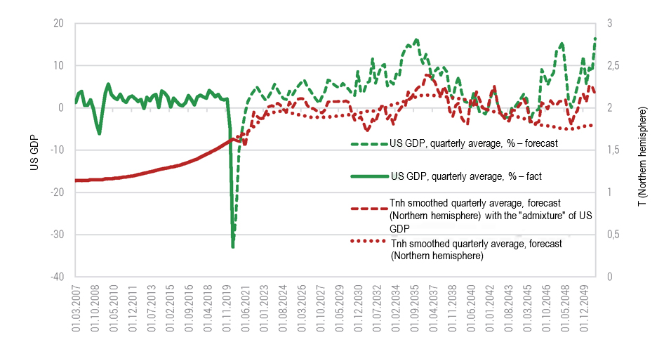
The performed correlation analysis (Fig. 4) showed that the temperature change in the Northern Hemisphere correlates with the graph of the economic dynamics of US GDP with the correlation coefficient R = 0.27. Therefore, in this work, a neural forecast of the economic dynamics of US GDP was made with the addition of Tnh, the results of which are shown in Fig. 6.
It can be seen from this graph that the US GDP curve has fairly high volatility with clearly pronounced crises in 2009, 2020, and projected economic downturns in the 2030s and 2041. The inter-crisis period, which is 10-12 years, coincides with the characteristic periods of the Sun’s activity; however, crises at this time interval fall at the minimum level of the Sun’s activity [6]. Whereas at earlier stages (before 2006), they coincided with the peaks of solar activity. This fact, unfortunately, has not yet received a proper explanation. Other important factors may influence the current and future dynamics of economic development. The curve of the economic dynamics of US GDP is given according to quarterly average data; therefore, the economic failures in mid-2020 are more pronounced. The inclusion in the forecasting algorithm of the Tnh anomaly indicator somewhat reduces this volatility, making the failure peaks of economic crises less pronounced. The results of neural forecasting of US GDP with the “mixing” of temperature data of Tnh anomalies make it possible to see that the green GDP curve is well correlated with the smoothed red trend curve of temperature anomalies. Obviously, the world’s largest economy, the United States, has a certain impact on the studied climatic parameters – therefore, when discussing global warming, it should be recognized that the United States, along with China, is mostly responsible for the temperature rise in the Northern Hemisphere of the planet (due to the more advanced level of its economy and greater man-made influence).

Conclusions

The obtained results of spectral analysis and neural forecasting allow us to conclude that there is a certain cyclical nature of natural and climatic phenomena. They can be treated as one of the macroeconomic indicators for the long-term forecasting of GDP dynamics. It was found that the level of correlation between temperature anomalies and an increase in the number of natural anomalies is considerably higher than the relationship between temperature anomalies and economic growth. However, there is also a visually and quantitatively statistically-significant relationship between global warming and economic dynamics (US GDP). In particular, accounting for the “mixing” of natural and climatic factors of economic indicators in the preparation of neural forecasts makes it possible to more accurately predict the onset of crisis phenomena in the economy. There are studies showing that an increase in temperature anomalies can lead to a long-term negative impact on economic growth [13], which in turn determines the importance of taking into account both the direct and inverse “economy – climate” relationship. Even given all the significance of human activities, its noospheric nature suggests that not only human activity transforms nature, but that the very nature of the Earth and space themselves determine the life of the economy and society. This is manifested, among other things, in the formation of cycles of economic and social life. New global challenges are associated not only with geopolitical confrontation, “bubbles” of the virtual economy and transformation of the world energy structure – but also with the growth of natural energy activity.

This work was financially supported by the Institute for Research and Expertise of VEB.RF and at the expense of the Russian Foundation for Basic Research (project No. 1805-60252).